Data Tables
Species Codes
POTR: Populus tremuloides, trembling aspen
POBA: Populus balsamifera, balsam poplar
POSP: Populus spp., uknown poplar species
PIGL: Picea glauca, white spruce
PIMA: Picea mariana, black spruce
Pinus: Pinus spp. (jack pine and lodgepole pine were grouped in this study)
BESP: Betula spp. (paper birch and Alaska birch were grouped in this study)
ABBA: Abies balsamea, balsam fir
Damage Codes:
FB: fungal fruiting bodies
SW: soft wood, indication of higher decay class/wood that has been dead a long time or fungal infection
DT: dead top (on live tree)
BT: broken top/snapped stem
Status:
L: live tree
D: dead tree
- Mortality rate is calculated by summing the total stems of decay class 1 and 2 and comparing this to total stem counts for each plot.
- Green table: mort=(sum_dead/total), where sum_dead only includes dead trees of decay class 1 and 2 and total includes all stems (regardless of live/dead status or decay classification)
- Orange table: sppmort=(sum_dead/totalspp), where sum_dead here only includes dead trees of decay class 1 and 2 within each species, and totalspp includes all stems of the species
Exploratory Visuals
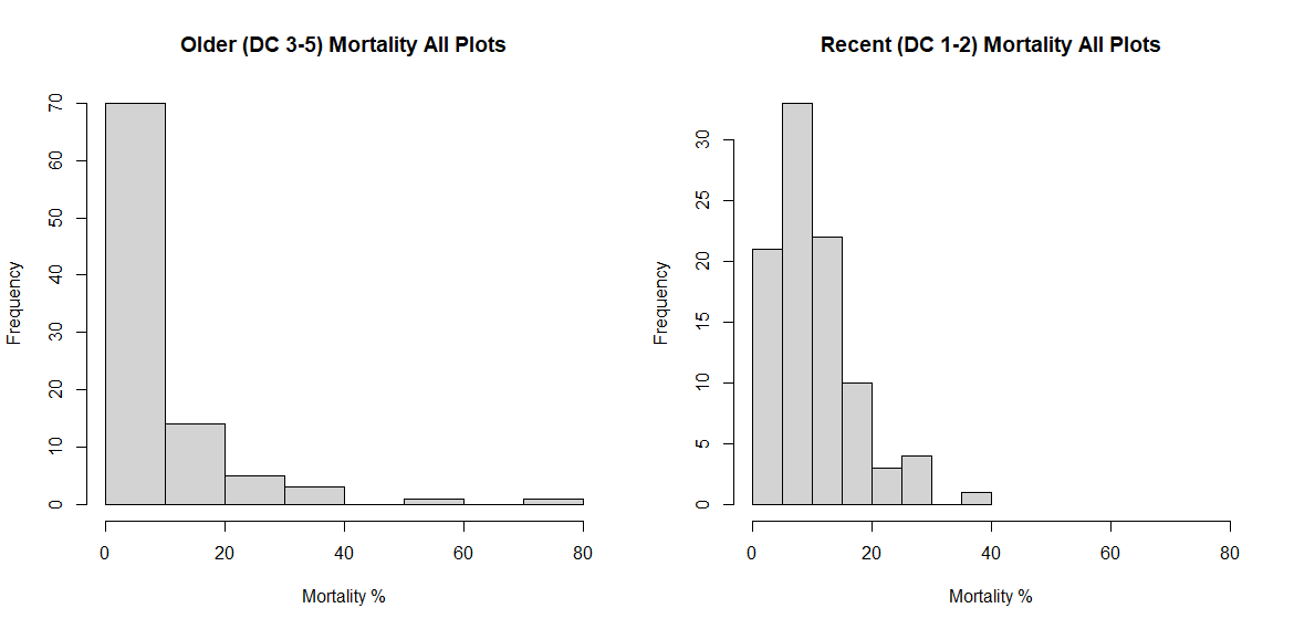
Fig. 8: distribution of mortality rates of both older dead and recent dead trees. Mortality rate is calculated by summing the total stems of decay class 1 and 2 and comparing this to total stem counts for each plot.
Looking at the distribution of mortality across all plots regardless of treatment type, we see that there was a shift towards higher mortality rates in the recent dead (decay class 1 and 2), which makes sense because we'd expect there to be an increase in mortality following the disturbance event.
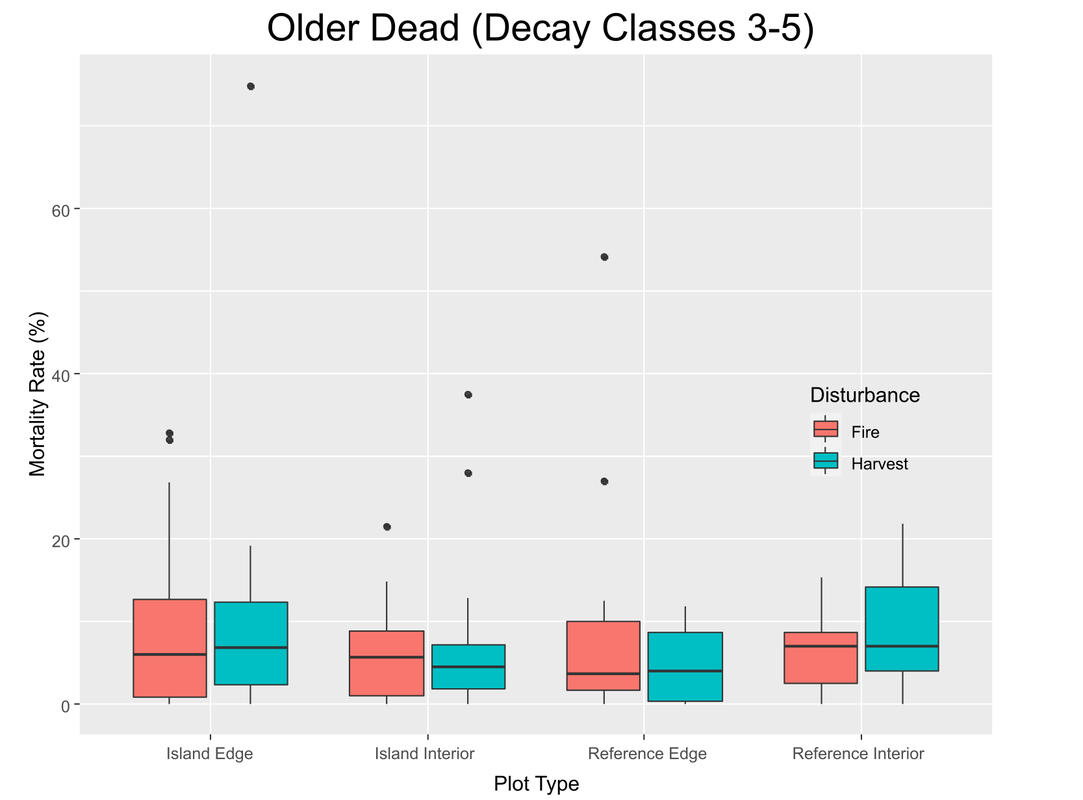
Fig. 9: mortality rate (%) of older dead (decay class 3-5) trees compared to total stems in all plot types and disturbance types. Mortality rate is calculated by summing the total stems of decay class 1 and 2 and comparing this to total stem counts for each plot.
|
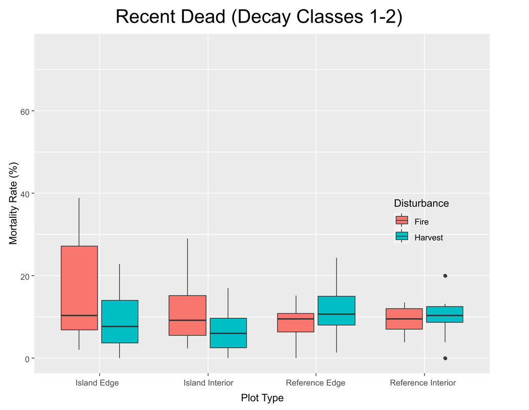
Fig. 10: mortality rate (%) of recent dead (decay class 1-2) trees in all plot types and disturbance types. Mortality rate is calculated by summing the total stems of decay class 1 and 2 and comparing this to total stem counts for each plot.
|
There is an increase in mortality amounts in all plots in both spread and median amounts for the recent dead. We also see that fire island edge plots have overall higher mortality than other plot types, fire island mortalities in both edge and interior plots are higher than in harvest-created islands and that in reference plots post-harvest disturbance shows slightly higher mortality than post-fire reference plots.
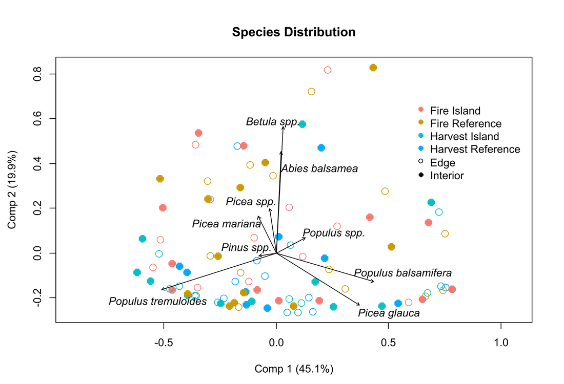
Fig. 11: principle component analysis of all stems of species distribution across all plots--this is not looking at mortality, just overall distribution of tree species across all plot types
This PCA shows species distribution (count of total stems) across disturbance type (fire and harvest) and location type (island and reference). We see that this ordination shows close to 65% of the variance, and that between the two disturbance types there aren't certain species strongly associated with either type of disturbance, and also the island and reference plots have similar species compositions. Birch (Betula spp.) and fir (Abies balsamea) are strongly correlated because the plots that had birch tended to also have fir, and these plots were overwhelmingly seen in the Flattop fire complex area.
Data Transformation
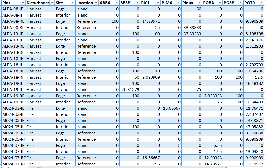
Fig. 12: example of species mortality data showing many zero values, to rationalize the Hellinger transformation of data to deal with the zero inflation
|
Because both the species stem counts and species mortality are zero inflated datasets, I transformed the data using the Hellinger transformation in the vegan package to account for the excess of zero values.
|
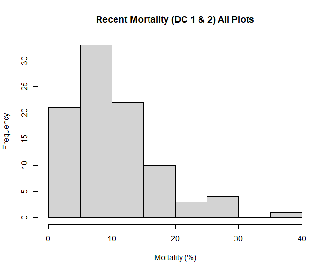
Fig. 13: recent mortality across all plot types, this distribution is skewed to the right and is not a normal distribution
|
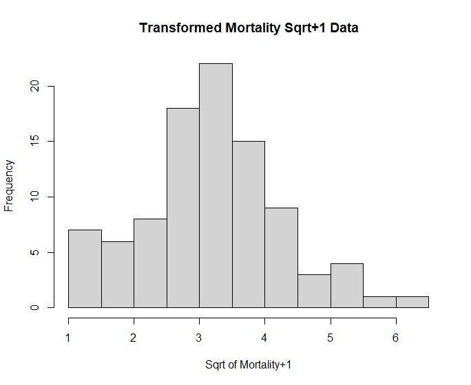
Fig. 14: mortality values were transformed with (sqrt mortality +1) to fit a more normal distribution
|
Recent mortality (decay classes 1 & 2) is skewed to the right, so doing a transformation of the data (taking the squareroot +1) gives a normal distribution to be used in univariate statistical analysis.
Modeling & ANOVA
Both fixed effects and mixed effects models were run with different error terms defined--primarily with a focus on "Block" being the harvest or fire area that plots were in--there were 6 of these blocks. The models were run with data that had been transformed to fit a normal distribution, and model assumptions were checked with plots of residuals to check homogeneity of variance and normality.
Models comparing mortality amounts:
-Model 1: Disturbance* Location=comparing Fire and Harvest Islands and References
-Model 2: Disturbance * Location*Site= comparing edge and interior plots of fire/harvest and reference/island
-Model 3: Disturbance*Site=comparing edge and interiors of fire and harvests (but not including island/reference plots)
-Model 4: Disturbance*Site*Area=comparing island size to fire and harvest edge and interiors (no reference plots included)
ANOVAs were run on all of these models to determine which treatments (if any) had significant effects on tree mortality amounts seen in different plots.
Assumptions of homogeneity of variance and normally distributed residuals were checked by plotting the models with plot() and qqnorm() functions in R.
Error Check
Looking at the distribution of mortality overall, there was one plot with a very high mortality ~80% (specifically in older decay classes). The majority of data analysis and visualization was done using a subset of decay classes and focusing on recent dead stems (decay classes 1 & 2), so this one plot's large mortality rate was left out of further data analysis and results.
